prior probability

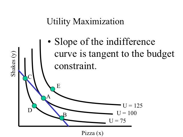
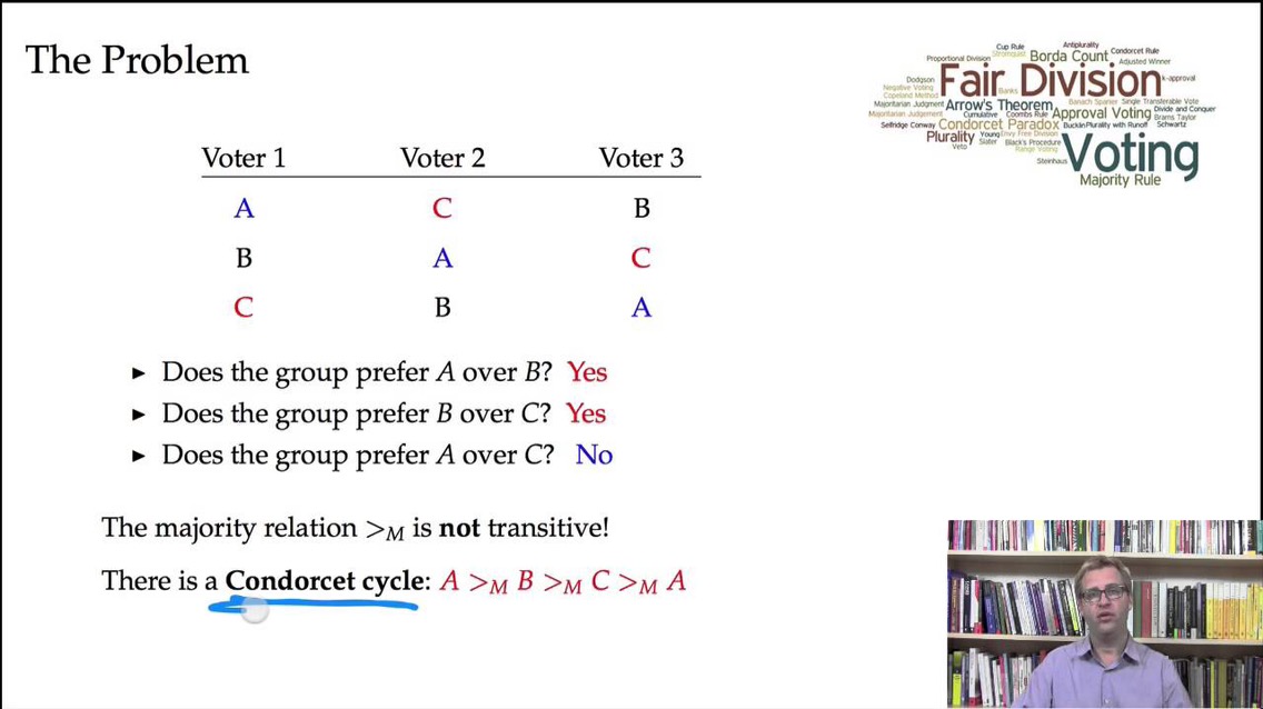
In our previous post, we proposed the possibility of a “contagion model” of legal evasion, noting that such a model is plausible given that people tend to copy or imitate what other people are doing. Here, we present the details of our model. We start with a finite population of actors consisting of some number of law evaders and of law abiders as follows:

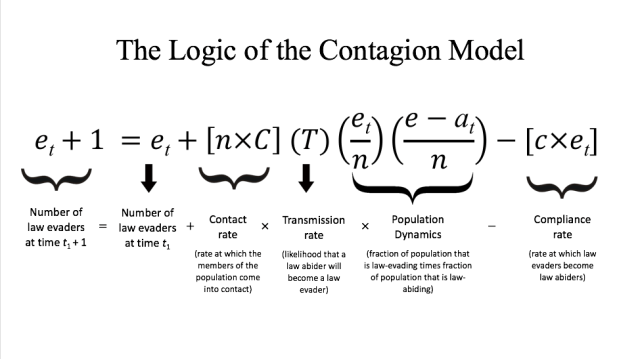
• Let n be number of people in a given population.
• Let e_t be the number of law evaders in population n at time t.
• Let n – e_t be the number of law abiders at time t.
• Let C (big C) be the level of contact between people in the population.
• Let Τ be the contagion or transmission rate; i.e. the likelihood that a law abider will become a law evader.
• And let c (little c) be the natural or constant level of compliance in the population.

As a result, c × e_t is the compliance rate; i.e. the rate at which law evaders become law abiders, and n × C is the contact rate; i.e. the rate at which the members of a population meet or come into contact with each other. (Note: the variable big C is what distinguishes our contagion model from information cascade models, which assume that the public behavior and decisions of all actors are common knowledge. In our contagion model, by contrast, each actor meets (and thus observes) a limited number of fellow actors, depending on the value taken by big C.)

Given these variables and parameters, we now present the logic of our contagion model as follows:

Thankfully, our contagion equation above can be simplified through algebraic manipulation as follows:

e_t + 1 = e_t + e_t × {C × T × [(n – e_t)/n] – c}

Notice that as the variable e_t approaches zero, the (n – e_t)/n term in the equation above approaches 1, so the model can be further simplified as follows:

e_t + 1 = e_t + e_t × [C × T – c]

As a result, our model tells us that law-evading behavior will spread when C times T > c. In words: when the contact rate times the transmission rate is greater than the rate of compliance, law-evading behavior will spread through the population because the number of law abiders changing their behavior as they come into contact with law evaders is greater than the natural rate of compliance in the population.

But what are the values for C, T, and c? Broadly speaking, we would expect these parameters to vary depending on the actual population of actors we are modelling. By way of example, we would expect big C, the level of contact, to be high in a mobile and modern population and low in a rural or pre-modern population. Moreover, we would expect T, the transmission rate, to vary depending on the ratio of law abiders to law evaders in the population, and we would expect little c, the level of compliance in a population, to depend (endogenously) on the general level of trust in a given population and (exogenously) on the levels of detection uncertainty as well as legal uncertainty. In our next post, we will consider the interaction between both types of uncertainty: detection uncertainty and legal uncertainty.

In our previous post, we commented on our colleague Alex Raskolnikov’s simple model of legal uncertainty in his excellent paper titled “Probabilistic Compliance” (Yale Journal on Regulation, 2017). To sum up, we loved his probabilistic model of compliance (in our view, it’s one of the best models of legal uncertainty we’ve studied so far, along with Mark Cronshaw and James Alm’s (Public Finance Quarterly, 1995) game-theoretic model of “two-sided uncertainty,” available here, via Research Gate), but we identified two potential blind spots in Raskolnikov’s elegant model. In brief, his model assumes away “detection uncertainty,” and in addition, like all maximization models, it assumes away the social dimension of compliance and evasion behaviors. Accordingly, I will take a different approach, one that emphasizes “probabilistic evasion” and one that models the social dimension of evasion. Specifically, what if law-evading behavior is more like an infectious disease, one that is capable of spreading across a population? (And just as important, what effect could legal uncertainty have on the rate of transmission?) A contagion model is plausible to the extent some (many?, most?) people tend to copy or imitate what other people are doing. Another advantage of a contagion model is that we don’t have to make any demanding common knowledge assumptions, unlike information cascade models that assume each actor is able to observe the choices and decisions made by all other actors. So fasten your seat belts: we will present our contagion model of evasion in our next blog post.

How fast does evasion spread?

Thus far, we have seen that many legal rules consist of general standards and thus generate some level of uncertainty. But is it possible to model this legal uncertainty or rule uncertainty in any formal or mathematical sense? In an excellent forthcoming paper titled “Probabilistic Compliance,” to be published in the Yale Journal on Regulation, Alex Raskolnikov, presents a probabilistic model of compliance. Raskolnikov is a professor of tax law at Columbia University, so he knows what he is talking about, and since his paper is one of the most intriguing works we have read on this subject, we shall summarize it here in some detail.

To begin with, his model has just five fundamental building blocks: x, C, b, F, and G.

• x is the level of compliance chosen by a regulated actor. In other words, when the law is uncertain, an actor in Raskolnikov’s model must decide how much time and resources to invest in its compliance efforts.
• C is the cost of figuring out and complying with an uncertain legal standard.
• b is the benefit from complying with the law, i.e. whatever penalty is avoided by complying with the law.
• F is the probability of obtaining this benefit. F is probabilistic precisely because the law is uncertain and the amount of compliance, variable. There is no guarantee that x compliance level will actually result in compliance.
• G is the actor’s expected gain, i.e. expected benefits minus expected costs.

Now, here is Raskolnikov’s model: G(x) = bF(x) minus C(x). What we love about this simple model is that G, F, and C are all a function of x, the actor’s compliance effort. In other words, F is a function of x because the greater an actor’s compliance efforts, the more likely he will be found in compliance. Likewise, C, the cost of compliance, is also a function of x, since stronger compliance positions generally cost more time and resources than weaker compliance positions. And lastly, because compliance is costly and because the level of compliance is variable, the expected gain of compliance is a function of x.

Another thing we love about Raskolnikov’s model is that it makes no reference to “social welfare.” Previous models of legal uncertainty generally assume there is some mythic and socially optimal set of legal rules (or some socially-optimal enforcement regime), but beyond crude guesswork, the social benefits and social costs of most legal rules (especially uncertain ones) are in reality almost always impossible to deduce or infer in any meaningful sense. For his part, Raskolnikov drops the social-optimality assumption altogether. Instead, his model attempts to figure out the optimal amount of compliance from an actor’s private or subjective point of view.

But as much as we love Raskolnikov’s simple model of probabilistic compliance, there are (alas) several serious problems with it. One is that he assumes that “detection and scrutiny are assured” (p. 112). (By the way, this is a problem that plagues previous models of legal uncertainty as well.) This assumption, however, cannot be right, since detection is probabilistic. Why, then, do Raskolnikov and others assume away detection uncertainty?

The other problem with most, if not all, previous models of legal uncertainty (including Raskolnikov’s)–and with previous models of detection uncertainty, for that matter–is that all these models are “maximization” models. That is, these models assume atomistic actors, all of whom are making their maximization calculations individually and in isolation from everyone else. In brief, these maximization models all assume that actors are perfectly interchangeable or perfectly fungible. If the values of each variable in a given maximization model are the same, then an actor will make the same decision, regardless of what other people are doing. But this too cannot be right. In reality, people’s decisions are very much influenced by what other people are doing. (This is why, for example, economists are unable to explain such a simple thing as the act of voting in national elections, which makes absolutely no sense from an economic point of view.)

In sum, we don’t mind it when economists have to posit perfectly rational actors. After all, they have to do this in order to make the mathematics of maximization work. What we do mind is positing perfectly atomistic actors instead of social actors. In the real world, many legal commands are not only uncertain; detection is also uncertain and actors’ compliance efforts are not atomistic but are instead influenced to some degree by the decisions made by other people. Given these truths (or at least axioms), I will present some alternative social models of legal compliance and legal evasion in my next few blog posts.

Does anyone really decide like this?

In our previous post, we mentioned the distinction between “detection uncertainty” and “legal uncertainty.” Briefly, detection uncertainty refers to the risk or probability of getting caught and punished; legal uncertainty, by contrast, occurs when there is no bright line separating compliance from noncompliance (cf. Raskolnikov, 2017, p. 104), as is often the case in law.

To provide some context, consider the “rule of reason” test used by courts in antitrust cases or the reasonable man test of tort law. Both legal tests consist of general standards and thus generate some level of legal uncertainty, since there is no clear cut dividing line between reasonable and unreasonable behavior in the domains of antitrust and accidents. (In the alternative, compare the NFL’s Rule 2–the rule Tom Brady was accused of violating, i.e. the rule relating to the amount of air pressure in a football, a clear and precise rule if there ever was one–with Rule 8–the complex and convoluted rule defining what a completed pass or “catch” is. Remember Dez Bryant’s controversial no-catch?) What effect does legal uncertainty have on the levels of compliance, evasion, and enforcement?

Thus, of the two kinds of uncertainty, the latter (legal uncertainty) is the more interesting and puzzling one. After all, one would expect higher levels of evasion the greater the level of detection uncertainty (i.e. the less likely one is of getting caught or punished), and vice versa, all other things being equal. But the ultimate effect of legal uncertainty on the levels of compliance and evasion (and on the level of enforcement for that matter) is less clear. Several scholars (mostly economists and tax lawyers) have attempted to solve this puzzle. We will discuss their work and delve into their formal models of legal uncertainty in our next few blog posts.

In our previous post, we asked: what is the optimal level of cheating in any given domain, such as business, dating, politics, sports, etc.? It turns out there is a long-standing literature on this problem, going back to such philosophical giants as Thomas Hobbes, Cesare Beccaria, and Jeremy Bentham. Broadly speaking, these great thinkers saw cheating and wrongdoing as a function of the probability of getting caught or punished for one’s misdeeds, so this tradition in political philosophy emphasizes the deterrent effect of law and social norms. In brief, the deterrence approach assumes that people decide whether to obey or evade the law or norms after rationally calculating the gains and consequences of their actions. The late Chicago economist Gary Becker revived this approach in the 1960s and 1970s, and since then, some of the best and brightest economists of our times have thought about this problem (compliance vs. evasion), modelling the decision whether to evade or comply as a form of decision-making under uncertainty. The source of the uncertainty varies in these second-generation models, depending on whether the law itself is unclear (legal uncertainty), or on whether enforcement is uncertain (detection uncertainty). We will discuss the difference between these two types of uncertainty in our next blog post.

Judit Veszeli

That is the subject of one of our ongoing research projects. Cheating occurs in many different domains: business, marriage, politics, sports, etc. In the business world, for example, fraud comes in many shapes and sizes, such as the massive manipulation of the London Interbank Offered Rate (the Libor scandal), the eggregious Volkswagen emission scandal, and the transnational FIFA corruption case. Are these business scandals rare outliers,  isolated incidents, or the tip of the iceberg? Stay tuned. We will be blogging about this question in the days ahead.

Jason Lundell

In our previous posts (starting with this one), we have proposed an alternative method of voting on multi-member courts. Broadly speaking, we would replace “one-judge, one-vote” with a method of “bayesian voting” in which judges would rate the legal arguments of the parties by disclosing their degrees of belief in the merits of those arguments. This method of voting goes by various names: range voting (Warren Smith), utilitarian voting (Claude Hillinger), score voting (Patrick Lundh), point voting (Hylland-Zeckhauser), and cardinal voting, just to name a few variants. We, however, prefer the term “bayesian voting” because we wish to emphasize the probabilistic and subjective nature of law in hard cases. Also, the label “bayesian voting” highlights a direct relation between our method of voting and the influential ideas about subjective probability developed by Frank P. Ramsey and Bruno de Finetti (pictured below). In brief, Ramsey and de Finetti were the first to propose a subjective definition of probability, now referred to as “Bayesian probability.” According to this Bayesian view, probability is not a property of the real world. Instead, probability is the subjective expression of your personal view of the world. Specifically, a statement’s probability is just a particular individual’s degree of belief in that statement. On this subjective view of probability, even if two people’s judgments about the probability of a statement or hypothesis are vastly different at time t₁, after evidence for (or against) the statement/hypothesis comes in at time t₂, rational people should then revise their degrees of beliefs. Moreover, their degrees of belief will tend to converge to the same probability as more and more evidence comes in. And isn’t this subjective convergence toward truth a good description of how the common law is supposed to work?

P.H.S. Torr

When the law is contested and a case is appealed to a higher court, the higher court must, at a minimum, make two decisions. First, it must decide whether the lower court committed any legal errors (Decision #1), and if so, it must decide secondly whether any of those legal errors are serious enough to warrant a reversal of the lower court’s decision (Decision #2). Formally, let’s call Decision #1 (did the lower court make a legal error?) the choice between e and not e, and let’s call Decision #2 (if there is an error, is it serious enough for a reversal?) the choice between small e and large e. For ease of exposition, let’s limit our discussion to Decision #1, the choice between e and not e. (The same logic applies to the choice between small e and large e.) Under the traditional method of judicial voting (one-judge, one-vote), the votes of each judge are equally weighted. Thus the “one-judge, one-vote” rule can only tell us whether e is ahead of not e (or vice versa). By contrast, under bayesian voting, judges would have to disclose their degrees of belief in e or not e. As a result, bayesian voting generates more information than simple majority rule vote: a bayesian voting procedure would reveal the comparative intensities of the judges’ beliefs about e and not e. Continue reading →

We’ve been blogging (on and off) about the possibility of “bayesian voting” on multi-member courts. The idea is to use a sliding scale (from 0 to 1) to allow each judge to express his degree of confidence (or credence) in the proper outcome of a case, instead of allocating a single up or down vote to each judge. Perhaps the most serious criticism against bayesian voting, however, is that it is anti-majoritarian, since it rejects the one-man, one-vote principle, specifically the one-judge, one-vote rule used by appellate courts. But the problem with one-man, one-vote is that majoritarian rule does not allow each judge to express the intensity of his beliefs in the proper outcome of a case. Furthermore, as William Riker and others have shown, majority rule produces incoherent results (see image below) and can be easily gamed to produce almost any outcome. In short, if we want to solve the paradoxes of voting that can occur in multi-member panels, then majority rule must give way to the “rule of credences.” We will explain why with a simple example in our next blog post.

Eric Parcuit

We interrupt our series of blog posts on bayesian voting to share the following link and table with our loyal followers: “There has been a long debate over single-payer versus multi-payer health insurance system. Which of these two systems is a better system? Some countries such as UK, Canada, and South Korea use single-payer system, whereas the U.S., Germany, and Japan rely on multi-payer system … [although] Medicare in the U.S. is indeed a single-payer health insurance for those aged 65 or older or those with disabilities….” (Source: Yusuke Tsugawa (津川  友介), via Health Policy Buzz Blog.)