prior probability

Some scholars are beginning to advocate for a partial lottery system for the awarding of research grants, an idea that is long overdue in my humble opinion. Why? Among other things, because under a random allocation system a new researcher would have just as much probability of winning an award as an established or big-name researcher does. (See links below for more details. Hat tip: The Amazing Tyler Cowen.)

1. James Urton, How economic theory and the Netflix Prize could make research funding more efficient, via UW News.
2. Kevin Gross & Carl T. Bergstrom, Contest models highlight inherent inefficiencies of scientific funding competitions, via PLOS Biology.
3. Ferric C. Fang & Arturo Casadevall, Research funding: the case for a modified lottery, via mBio.
    

Credit: Fang & Casadevall

President Trump wants Congress to fund a border wall; the Democrats, who now have regained control of the House of Representatives, do not want to fund a border wall. Which side will “swerve” first? The Game of Chicken, along with the Prisoner’s Dilemma and the Battle of the Sexes, is one of the ways in which this political conflict can be modeled. Here is the Wikipedia entry for the Game of Chicken; here is a memorable example of Chicken from the movie “Footloose”.

Bayesian Update (6pm/18h): As I replied to Kathy H. in the comments section, I find it fascinating that in this particular case the intransigence of both sides is due to their moralizing of the border wall, which suggests an inverse relationship between the ability to reach a pragmatic compromise and the strength of one’s moral convictions!

We have been attending the 21st Annual Federalist Society Faculty Conference in New Orleans, where we presented our work in progress “Bayesian Stare Decisis.” Shout out to Gene Meyer, the president of FedSoc, for hosting an excellent conference. Unlike the elitist AALS conference next door, the Federalist does not charge any fees and is open to legal scholars of all political persuasions.

While I was attending and live-tweeting a scholarly panel on “substantive due process” at this year’s Federalist Society Faculty Conference, a colleague of mine penned the beautiful doodle pictured below.

Artist Unknown. Photo Credit: F. E. Guerra-Pujol.

My wife Sydjia found this stop sign on the corner of Dante and Freret streets in New Orleans.

Photo credit: F. E. Guerra-Pujol

We recently visited The James Museum of Western & Wildlife Art, which is located in St Petersburg, Florida. Enjoy! 

“Coors is the one” by John Nieto (1988)

Note (1/4): This post has been significantly revised.

In our previous post, we used Bayesian reasoning to revise or “update” our forecast about the possible outcomes in Gamble v. United States, a case that was heard by the Supreme Court of the United States (SCOTUS) on 6 December 2018 and that as of today (31 December) is still pending. In particular, based on the high number of amicus briefs submitted to SCOTUS in this case, we concluded there is a 37% probability that SCOTUS will overrule the “separate sovereigns” doctrine when it announces its decision sometime in 2019.

But how can we tell whether our forecast is a good one or not? Standing alone, we cannot. Either SCOTUS will or will not change the jurisprudential status quo when it decides Gamble. But when we are able to make many probabilistic forecasts–i.e. when we forecast the outcomes of a large number of cases–we can then measure or score the accuracy of our forecasting methods using a scoring method that was first proposed by Glenn Wilson Brier, who was an early advocate of probability forecasting and the use of probability forecasts in decision making. (See Glenn W. Brier, “Verification of forecasts expressed in terms of probability,” Monthly Weather Review, Vol. 78, no. 1 (1950), pp. 1-3. For more biographical details about Brier’s life and forecasting work, see here.)

In its simplest formulation, Brier’s simple scoring method produces a “Brier score” as follows:

Brier Score = 1/N ∑ (f_x – o_x)²

where N is the total number of forecasts, f_x is the probability that was forecast, and o_x is the outcome of the binary event that was the subject of the forecast. Before proceeding, it is worth noting that the value for f_x must always be expressed in the range of 0 to 1 and that the value for o_x must be either 0 or 1: zero if the event does not happen and 1 if it does happen. (The subscript x is just a gentle reminder that the accuracy of a set of predictions will be unknown until the events being forecast take place or not.)

In plain English, the Brier score attempts to quantify the accuracy of a set of probabilistic predictions of binary events by measuring the mean squared error of each prediction. Using this simple formulation, this score will take on a value somewhere between 0 and 1, since this range is the largest possible difference between a predicted probability f_x, which must be between 0 and 1, and the actual outcome o_x, which can take on values of only 0 or 1. The lower the Brier score is for a set of predictions, the more accurate those predictions are as a whole. (In Brier’s original formulation of his scoring method, the range is from 0 to 2. Tetlock and Gardner offer a good explanation of the logic of Brier’s scoring method on pp. 59-66 of their “superforecasting” book.)

We can illustrate this ingenious scoring method by returning to our initial example, the aptly-named case of Gamble v. United States. Taking into account the number of amicus briefs that were submitted in this case, we reasoned there is a 37% probability (f_x = 0.37) that SCOTUS will overrule the “separate sovereigns” doctrine when it decides Gamble. Therefore, if this unlikely event were to occur, o_x will assume the value 1; if it does not occur, o_x is zero. Given this prediction, my Brier score for this forecast can be calculated as follows: (1) if SCOTUS does decide to overrule itself in Gamble, my Brier Score is going to be (0.37 – 1)² = (– 0.63)² = 0.3969; (2) if, however, SCOTUS decides to not overrule the precedent, my Brier Score is (0.37 – 0)² = (0.37)² = 0.1369. [*]

Notice that my Brier score is higher when SCOTUS does not change the jurisprudential status quo, i.e. when it does not overrule its precedents. Why? Because saying there is 37% probability that an event x will happen (e.g. a change in the status quo) is equivalent to saying there is a 63% that x will not happen (e.g. the status quo will remain), so I should receive a higher score if x does not happen. That said, a single forecast is not enough to measure my forecasting acumen. To truly measure the forecasting accuracy of my Bayesian methods (and of my use of amicus briefs as a proxy for whether the status quo will change or not), we must make a large number of forecasts. For instance, if my Bayesian prediction model is a good one, SCOTUS will change the status quo close to 37% of the time in the entire population of cases in which my model predicts such a change. We will thus assemble a larger database of cases with which to test our model, and we will report our results in a future post. In the meantime, Happy New Year!

Source: David Lowe (Scrum & Kanban)

Continue reading →

Note (1/4): This post has been significantly revised.

In our previous post, we painstakingly estimated the base rate or the historical frequency in which a precedent is overturned by the Supreme Court of the United States (SCOTUS) in those cases in which a party is asking SCOTUS to take such an action. In short, since 2005, the year John Roberts was appointed and confirmed as Chief Justice, we estimated a 13% or 0.13 prior probability that SCOTUS will change the “jurisprudential status quo” by overturning a precedent in the smaller subset of cases in which a party is asking SCOTUS to overrule one or more of its precedents.

Now that we have established our base rate, we can forecast how likely it is that SCOTUS will overrule one of its own decisions in any particular case this term. By way of example, let’s consider the aptly-named Gamble v. United States, docket number 17-646, which was heard by SCOTUS on 6 December 2018. As of today (30 December), a decision in this case is still pending. In summary, the attorneys for the petitioner, Mr Terance Gamble, are asking SCOTUS to overrule the “separate sovereigns” exception to the Double Jeopardy Clause, which would require SCOTUS to overrule a line of precedents culminating in Abbate v. United States, 359 U.S. 187 (1959). How likely is it that SCOTUS will overrule this doctrine?

Historically speaking, there is only a 0.13 chance such a dramatic event will occur. Given such a modest base rate, without any additional information we might be tempted to conclude that it is unlikely that SCOTUS will depart from its previous precedents when it decides Gamble. Nevertheless, it turns out that a substantial number of amicus briefs were submitted in this case: 12 in all, or just a shade more than the historical average of 11.75 amicus briefs per case since 2010. Given this new piece of information, we can now use Bayesian reasoning to update our prior! Specifically, the Bayesian approach to forecasting requires us to estimate two sets of conditional probabilities. One is the hit rate or p(E|H): the likelihood of seeing a high number of amicus briefs (with “high” defined as any number greater than the historical average of 11.75 amicus briefs per case) when SCOTUS decides to change the status quo by overturning a precedent or declaring a federal law unconstitutional. The other is the miss rate or p(E|not H): the likelihood of seeing a high number of amicus briefs even when SCOTUS decides to uphold the status quo, i.e. when SCOTUS does not overturn a precedent or does not strike down a federal law.

Next, let’s estimate these two sets of probabilities for the Roberts Court era: 2005 to the present. (Note: I am just going to guess what these probabilities are for now. As I mentioned in my previous post, I intend on applying for a research grant so I can comb SCOTUS’s records and determine what these probabilities are.) Let’s start with p(E|H). Surprisingly, not all cases that end up changing the jurisprudential status quo have generated a high number of amicus briefs. By way of example, there were only three amicus briefs in Montejo v. Louisiana, 557 U.S. 778 (2009), which overruled Michigan v. Jackson, 475 U.S. 625 (1986), and similarly, there were only four amicus briefs in Johnson v. United States, 556 U.S. ___ (2015), which struck down a portion of the federal Armed Career Criminal Act. Nevertheless, most cases that end up departing from the jurisprudential status quo do tend to generate a high number of amicus briefs, so let’s assume that 20 out of the 25 Roberts Court cases that did change the status quo also generated a high number of briefs. (Stated formally, p(E|H) = 0.8.)

But at the same time, we should also expect to see a high number of amicus briefs even when SCOTUS decides to uphold the status quo, so let’s assume that only one of every five cases with high numbers of amicus briefs (i.e. greater than 11.75) will depart from the jurisprudential status quo, i.e. will involve a decision overturning a precedent or striking down a federal law. (Stated formally, p(E|not H) = 0.2.) Now all that remains for us to do is to plug these three probability estimates (base rate, the hit rate, and miss rate) into Bayes’ formula, which is pictured below. In plain English, the updated probability p(H|E) that SCOTUS will change the status quo when it decides Gamble is the hit rate times base rate divided by the hit rate times base rate plus the miss rate times one minus the base rate. When we plug our guesses into Bayes’ formula, we see there is now a 37% probability that SCOTUS will overrule the “separate sovereigns” exception to the Double Jeopardy Clause. Although 37% is still a modest probability, it is almost three times as high than our historical base rate of 13%!

But how can we know whether this forecast is a good one or not? In my next post, I will steal another idea from Tetlock and Gardner’s 2015 excellent “superforecasting” book to answer this question: the idea of the Brier score. The basic idea is this: once we make a large number of SCOTUS forecasts, we will be able to score the overall accuracy of my simple forecasting model.

Source: Norman Fenton

Continue reading →

Note (1/4): The second half of this post has been significantly revised.

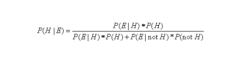
We have been highlighting some of the main ideas contained in Tetlock and Gardner’s 2015 “superforecasting” book in our previous two blog posts. Yesterday, for example, I presented a step-by-step overview of their Bayesian approach to forecasting. In my next two posts, I will restate Tetlock and Gardner’s Bayesian methodology in formal mathematical notation (see image below) and present a concrete example relevant to my domain of expertise (constitutional law).

In particular, I would love to be able to forecast when the Supreme Court of the United States (SCOTUS) is going to overturn a precedent or when it is going to declare a law unconstitutional. In order to engage in Bayesian reasoning in this domain, i.e. in order to make a Bayesian forecast, we will need three pieces of information: (1) the “base rate” or the historical frequency p(H) in which precedents have been overturned in the past or in which federal laws have previously been declared unconstitutional; (2) some piece of evidence E, such as a large number of amicus briefs submitted to SCOTUS, that we are likely to see when a law or precedent is destined to be overturned, or p(E|H); and last but not least, (3) the probability or likelihood of seeing this same piece of evidence, i.e. a large number of amicus briefs, in those cases in which a precedent is upheld, or p(E|not H).

(Before proceeding, you should be asking, Why should the number of amicus briefs be considered a relevant piece of evidence when we are engaged in judicial forecasting? In brief (pun intended), it turns out there is a large scholarly literature attempting to measure the influence of amicus briefs on judicial decision making. I will review this fascinating literature in a separate post. For now, however, the fact that such an amicus practice exists and that there is such a large literature about this practice are, by themselves, relevant pieces of evidence that amicus briefs are important.)

How would we begin to engage in Bayesian reasoning in this domain? First, let’s start with the base rate. Since SCOTUS was created in 1789, it has heard over 28,000 cases! (Today, SCOTUS hears about 80 cases per term, with each Supreme Court Term commencing on the first Monday of October and concluding on the last week of June.) During this 230-year span, SCOTUS has overruled itself 236 times (here is a comprehensive list of “Supreme Court decisions overruled by subsequent decision“) and has found 182 federal laws to be unconstitutional (here is a list of “Acts of Congress held unconstitutional in whole or in part by SCOTUS“). These initial observations thus appear to indicate an extremely low base rate of 0.015 (rounded up), or 236 + 182 = 418 divided by 28,000.

Next, since the use of amicus briefs has become a regular practice only recently, let’s tinker with our historical base rate to make it more accurate. Specifically, let’s consider limiting our evidence to the recent past, say the period from the 2005-06 Term, when John Roberts replaced the late William Rehnquist as Chief Justice of SCOTUS, to the end of the 2017-18 term last year. (By 2005, the practice of amicus briefs in SCOTUS had become quite common.) During this shorter span of time (2005 to 2018), SCOTUS heard about 1000 cases, and by my count, the Roberts Court has decided 13 cases in which it overruled one or more of its precedents and has struck down 26 federal laws, either in whole or in part, or an average of two federal laws struck down per year. (Shout out to Professor Jonathan H. Adler for compiling these data!) These observations give us a revised base rate of 0.04, or 40 divided by 1000–still small, but almost three times as large as our previous base rate.

Notice that the base rate, standing alone, indicates that the reversal of a precedent or a judicial declaration that a law is unconstitutional is an extremely rare event, but its probability is not zero. In fact, the base rate could even be higher, since we should exclude the vast majority of cases in which none of the parties are asking SCOTUS to change the jurisprudential status quo. After all, asking SCOTUS to take such dramatic action as overruling a precedent or striking down a federal law is a long shot. Given this reality of appellate practice, let’s assume that the parties have asked SCOTUS to change the status quo in only 100 of the 1000 cases SCOTUS has heard from 2005 to 2018. (Note: this is just a simplifying assumption on my part. I intend on applying for a research grant to actually count up the number of times since 1789 that a lawyer has requested SCOTUS to change the jurisprudential status quo.)

This simplifying assumption will thus cause our revised base rate to increase up to 40 percent (!), or 0.4 (40 divided 100). This increase makes sense, since we have narrowed down the base rate to the smaller subset of cases in which one of the parties is asking SCOTUS to change the status quo by overruling a precedent or by striking down a federal law. But at the same time, the base rate is too high because it lumps together two types of cases: (1) cases in which a precedent is overruled, and (2) cases in which a federal law is declared unconstitutional. For the remainder of this post, let’s focus on the first type of case only. (Full disclosure: the stability of SCOTUS’s precedents is what motivated to engage in this research in the first place.)

Since there are only 13 Roberts Court cases in which a precedent was overruled, our revised base rate is 0.13, or 13 divided by 100. Now that we have a plausible base rate, we must next proceed to revise or “update” our historical base rate upon the arrival of new evidence. When SCOTUS agrees to hear a new case, for example, many government agencies, interest groups, and other non-parties will have an opportunity to present amicus briefs to the Court. In fact, it turns out that the median or average number of amicus briefs submitted to SCOTUS since 2010 is about 11.75 per case (see here, for example), but we should expect a greater number of amicus briefs the more important the case, i.e. the more likely the case has national or even international implications. In my next post, we will use this information (the number of amicus briefs) to predict the posterior probability that a precedent will be overturned.

Image credit: Kara Lilly, via mawer.com